在本章中,我们将重点关注我们将要从已知的一组点x和f(x)中学习的网络.一个隐藏层将构建这个简单的网络.
感知器隐藏层解释的代码如下所示 :
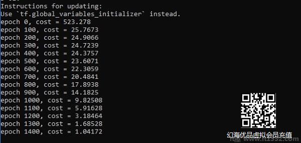
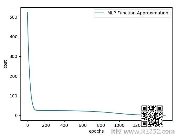
#Importing the necessary modules import tensorflow as tf import numpy as np import math, random import matplotlib.pyplot as plt np.random.seed(1000) function_to_learn = lambda x: np.cos(x) + 0.1*np.random.randn(*x.shape) layer_1_neurons = 10 NUM_points = 1000 #Training the parameters batch_size = 100 NUM_EPOCHS = 1500 all_x = np.float32(np.random.uniform(-2*math.pi, 2*math.pi, (1, NUM_points))).T np.random.shuffle(all_x) train_size = int(900) #Training the first 700 points in the given set x_training = all_x[:train_size] y_training = function_to_learn(x_training)#Training the last 300 points in the given set x_validation = all_x[train_size:] y_validation = function_to_learn(x_validation) plt.figure(1) plt.scatter(x_training, y_training, c = 'blue', label = 'train') plt.scatter(x_validation, y_validation, c = 'pink', label = 'validation') plt.legend() plt.show()X = tf.placeholder(tf.float32, [None, 1], name = "X")Y = tf.placeholder(tf.float32, [None, 1], name = "Y")#first layer #Number of neurons = 10 w_h = tf.Variable( tf.random_uniform([1, layer_1_neurons],\ minval = -1, maxval = 1, dtype = tf.float32)) b_h = tf.Variable(tf.zeros([1, layer_1_neurons], dtype = tf.float32)) h = tf.nn.sigmoid(tf.matmul(X, w_h) + b_h)#output layer #Number of neurons = 10 w_o = tf.Variable( tf.random_uniform([layer_1_neurons, 1],\ minval = -1, maxval = 1, dtype = tf.float32)) b_o = tf.Variable(tf.zeros([1, 1], dtype = tf.float32)) #build the model model = tf.matmul(h, w_o) + b_o #minimize the cost function (model - Y) train_op = tf.train.AdamOptimizer().minimize(tf.nn.l2_loss(model - Y)) #Start the Learning phase sess = tf.Session() sess.run(tf.initialize_all_variables()) errors = [] for i in range(NUM_EPOCHS): for start, end in zip(range(0, len(x_training), batch_size),\ range(batch_size, len(x_training), batch_size)): sess.run(train_op, feed_dict = {X: x_training[start:end],\ Y: y_training[start:end]}) cost = sess.run(tf.nn.l2_loss(model - y_validation),\ feed_dict = {X:x_validation}) errors.append(cost) if i%100 == 0: print("epoch %d, cost = %g" % (i, cost)) plt.plot(errors,label='MLP Function Approximation') plt.xlabel('epochs') plt.ylabel('cost') plt.legend() plt.show()输出
以下是函数的表示层近似 :
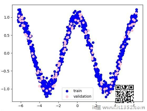
这里有两个数据表示W的形状.两个数据是:训练和验证,用不同的颜色表示,如图例部分所示.